In [3]:
## Sorry, this is an easier way to display a gif in HTML generated from a Python notebook
from IPython.display import HTML
HTML('<img src="https://miro.medium.com/v2/resize:fit:1400/1*ubRrYAZJUlCcqg7WoKjLgQ.gif">')
Out[3]:
This lab covers the construction, fitting, and evaluation of convolutional neural networks (CNN) using torch. You should begin by loading the following libraries:
import torch
import torchvision
import numpy as np
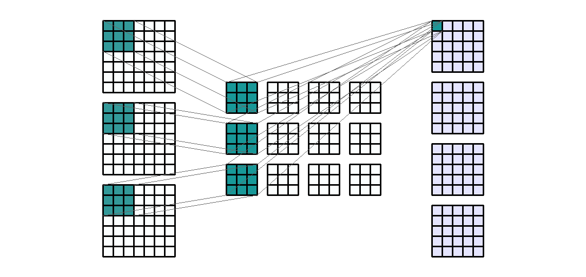
Convolutional neural networks can be viewed as an extension of the basic network architectures discussed in our previous lab involving hidden layers that perform new types of operations. The most important of these are convolutional layers, which we will implement using the Conv2d building block in torch.
The example below demonstrates the four essential arguments of Conv2d on a randomly generated tensor whose dimensions can be taken to reflect a single 7x7 image with 3 color channels:
## Create random tensor to represent a 7x7 image with 3 channels
random_tensor = torch.rand(1,3,7,7)

## Use random_tensor as input into Conv2d
from torch import nn
trial_net = nn.Conv2d(in_channels=3, out_channels=4, kernel_size=3, stride=1)
trial_output = trial_net(random_tensor)

## Check output shape
print(trial_output.shape)

## Check weights shape
print(trial_net.weight.shape)

## Check bias shape
print(trial_net.bias.shape)
torch.Size([1, 4, 5, 5])
torch.Size([4, 3, 3, 3])
torch.Size([4])
This example applied a set of 3x3 convolution filters using a stride length of 1 to our 1x3x7x7 input tensor. A few things to note:
in_channels must match the number of channels present in the input (generally this is the second dimension of the input tensor).out_channels determines the number of feature maps (output channels) to be produced by the layer. Specifying more output channels will increase the number of hidden features learned in this layer of the network.kernel_size determines the size of the filter, with kernel_size=3 indicating a 3x3 filter size. Note that you could provide a non-square filter by supplying a tuple, such as (2,3).Summarizing this operation, the 1x3x7x7 input tensor was convolved into 1x4x5x5 output tensor (note that we did not use any padding).
Because the input had 3 channels and we requested 4 output channels, our model must estimate weights for 12 different 3x3 filters, and 4 biases (1 per output channel). To better understand the role of these weights and biases, consider the following:
[1,:,:] of trial_net.weight, act seperately on the input channels to contribute, with the bias [1], to the first output channel.[2,:,:], act seperately on the input channels to contribute, with the bias [2], to the second output channel.The mechanics of this layer are displayed visually in the .gif below:
## Sorry, this is an easier way to display a gif in HTML generated from a Python notebook
from IPython.display import HTML
HTML('<img src="https://miro.medium.com/v2/resize:fit:1400/1*ubRrYAZJUlCcqg7WoKjLgQ.gif">')
Printed below are the first set of weights:
trial_net.weight[1,:,:]
tensor([[[ 0.0967,  0.0033,  0.1359],
         [-0.0457, -0.1048, -0.0194],
         [-0.1064,  0.1163,  0.1190]],

        [[-0.1144,  0.1168, -0.1006],
         [-0.0906,  0.1913, -0.0713],
         [ 0.0328,  0.0790,  0.0957]],

        [[-0.1570,  0.0912, -0.1159],
         [ 0.1386, -0.0825,  0.0475],
         [-0.0678, -0.0566, -0.0273]]], grad_fn=<SliceBackward0>)
Suppose a training example from the Fashion MNIST data (introduced in the previous lab) is given as the input to a convolutional layer created using Conv2d involving convolution kernels of size 4x4 and stride of 2.
Convolutional layers are used to learn spatially dependent feature patterns in an image. For example, the first convolutional layer in a deep network might detect edges, curves, and color gradients. However, it is easy for convolutional layers to produce output that is substantially larger than than is desirable. For example, if the input is padded and 10 convolution kernels are used to learn features from an image with a single input channel, the output tensor is now 10 times larger than the input.
Consequently, most convolutional networks use a pooling layer immediately after convolution to reduce the dimension of inputs into subsequent layers. As a demonstration, consider a randomly generated tensor of dimension [1,1,4,4]:
random_tensor = torch.rand(1,1,4,4)
print(random_tensor)
tensor([[[[0.8892, 0.0091, 0.6755, 0.4736],
          [0.6761, 0.7187, 0.3776, 0.3354],
          [0.6368, 0.5166, 0.9557, 0.8515],
          [0.7688, 0.9752, 0.5153, 0.7582]]]])
Sliding a 2x2 pooling filter across the 4x4 slice of this tensor using a stride of 2 creates 4 distinct regions, and pooling using MaxPool2d will keep only the maximum value within each region:
trial_pool = nn.MaxPool2d(kernel_size = 2, stride = 2)
pool_output = trial_pool(random_tensor)
print(pool_output)
tensor([[[[0.8892, 0.6755],
          [0.9752, 0.9557]]]])
Similarly, we could perform average pooling:
avg_pool = nn.AvgPool2d(kernel_size = 2, stride = 2)
pool_output = avg_pool(random_tensor)
print(pool_output)
tensor([[[[0.5733, 0.4655],
          [0.7244, 0.7702]]]])
Note that stride of 2 might be problematic for an input slice with an odd number of rows and/or columns. The default behavior in these situations is controlled by the argument ceil_mode. When set to False, the pooling filter cannot go "out of bounds", so certain portions of the input won't be used. When this argument is set to True, the filter can go out of bounds so long as its left corner starts in the input (or its left padding).
Consider the example below:
## Randomly generated 1x5x5 tensor
random_tensor = torch.rand(1,1,5,5)

## Two different pooling operations
ceil_false = nn.MaxPool2d(kernel_size = 2, stride = 2, ceil_mode = False)
ceil_true = nn.MaxPool2d(kernel_size = 2, stride = 2, ceil_mode = True)

## Note the difference in output shape
print(ceil_false(random_tensor).shape)
print(ceil_true(random_tensor).shape)
torch.Size([1, 1, 2, 2])
torch.Size([1, 1, 3, 3])
trial_output, produced in Part 1, apply ReLU activation followed by max pooling and note the output. Then, swap the order of these operations (ie: apply max pooling followed by ReLU activation). What impact does the order have on the output? At any step of a convolutional neural network we may apply padding to the input to help ensure that features present in the edges of the input are properly handled. While not an essential step, padding is usually applied to the inputs of a network's first convolutional layer, and sometimes to the inputs of subsequent layers.
For illustrative purposes, let's apply padding to the input tensor used in the pooling examples from the previous section:
## Randomly generated 1x5x5 tensor
random_tensor = torch.rand(1,1,5,5)

## Add padding
padding_step = nn.ZeroPad2d(padding=1)
padded_input = padding_step(random_tensor)
print(padded_input)

## See the impact
print(ceil_false(padded_input))
print(ceil_false(random_tensor))
tensor([[[[0.0000, 0.0000, 0.0000, 0.0000, 0.0000, 0.0000, 0.0000],
          [0.0000, 0.3443, 0.2315, 0.0039, 0.4375, 0.4186, 0.0000],
          [0.0000, 0.0356, 0.5737, 0.1951, 0.0751, 0.9896, 0.0000],
          [0.0000, 0.4622, 0.6268, 0.4209, 0.1618, 0.8350, 0.0000],
          [0.0000, 0.0370, 0.7792, 0.1690, 0.7236, 0.1897, 0.0000],
          [0.0000, 0.1471, 0.4918, 0.5798, 0.9537, 0.3755, 0.0000],
          [0.0000, 0.0000, 0.0000, 0.0000, 0.0000, 0.0000, 0.0000]]]])
tensor([[[[0.3443, 0.2315, 0.4375],
          [0.4622, 0.6268, 0.9896],
          [0.1471, 0.7792, 0.9537]]]])
tensor([[[[0.5737, 0.4375],
          [0.7792, 0.7236]]]])
Notice how padding allows our 2x2 pooling operation to consider the values stored in every element of the input tensor in this example. The tradeoff is that the output feature map is now slightly larger.
At this point we've covered the basics of how convolution, pooling, and padding operations are implemented in PyTorch. We're now ready to build a relatively simple convolutional neural network to use on the Fashion MNIST data (introduced in our previous lab).
Recall that this dataset contained 1000 examples (900 in the training set) of 28x28 pixel grayscale images of 10 different fashion objects.
We'll start by defining the network architecture:
from torch import nn

class my_net(nn.Module):

    ## Constructor commands
    def __init__(self):
        super(my_net, self).__init__()

        ## Define architecture
        self.conv_stack = nn.Sequential(
            nn.Conv2d(1,10,4,1),
            nn.ReLU(),
            nn.MaxPool2d(2,2),
            nn.Conv2d(10,30,2,1),
            nn.ReLU(),
            nn.MaxPool2d(2,2),
            nn.Flatten(),
            nn.Linear(750, 250),
            nn.ReLU(),
            nn.Linear(250, 10)
        )

    ## Function to generate predictions
    def forward(self, x):
        scores = self.conv_stack(x)
        return scores
nn.Conv2d(1,10,4,1) in the first convolution operation of the network? What are the dimensions after nn.ReLU() and nn.MaxPool2d(2,2) have been applied to this output?nn.Conv2d(1,10,4,1) so long as they contain a single color channel. Does this mean that this network architecture can handle input images of any size? Briefly explain.nn.Linear(750, 250) come from? Can the network still be used on the Fashion MNIST data (in its orginal format) if this value is changed?nn.Linear(750, 250) be changed without requiring changes to the format of the input data? Briefly explain.Next, we'll set up a few of the parameters required to train our network:
## Hyperparms
epochs = 300
lrate = 0.025
bsize = 100

## For reproduction purposes
torch.manual_seed(7)

## Cost Function
cost_fn = nn.CrossEntropyLoss()

## Intialize the model
net = my_net()

## Optimizer (Stochastic Gradient Descent)
optimizer = torch.optim.SGD(net.parameters(), lr=lrate)
Now we'll prepare the Fashion MNIST data to be used to train the network, this code should be familiar from our previous lab.
### Read flattened, processed data
import pandas as pd
fash_mnist = pd.read_csv("https://remiller1450.github.io/data/fashion_mnist_train.csv")

## Train-test split
from sklearn.model_selection import train_test_split
train_fash, test_fash = train_test_split(fash_mnist, test_size=0.1, random_state=5)

### Separate the label column (outcome)
train_y = train_fash['y']
train_X = train_fash.drop(['y'], axis=1)
test_y = test_fash['y']
test_X = test_fash.drop(['y'], axis=1)

### Convert to numpy array then reshape to 900 by 28 by 28
mnist_unflattened = train_X.to_numpy()
mnist_unflattened = mnist_unflattened.reshape(900,28,28)

## Convert to tensor
mnist_tensor = torch.from_numpy(mnist_unflattened)
train_X = torch.reshape(mnist_tensor, [900,1,28,28])

## Make DataLoader
from torch.utils.data import DataLoader, TensorDataset
y_tensor = torch.Tensor(train_y)
train_loader = DataLoader(TensorDataset(train_X.type(torch.FloatTensor),
                        y_tensor.type(torch.LongTensor)), batch_size=bsize)
We've now set up everything we'll need to train the network. We'll do so using the same training loop that appeared in our previous lab:
## Initial values for cost tracking
track_cost = np.zeros(epochs)
cur_cost = 0.0

## Loop through the data
for epoch in range(epochs):

    cur_cost = 0.0
    correct = 0.0

    ## train_loader is iterable and numbers knows the batch
    for i, data in enumerate(train_loader, 0):

        ## The input tensor and labels tensor for the current batch
        inputs, labels = data

        ## Clear the gradient from the previous batch
        optimizer.zero_grad()

        ## Provide the input tensor into the network to get outputs
        outputs = net(inputs)

        ## Calculate the cost for the current batch
        ## nn.Softmax is used because net outputs prediction scores and our cost function expects probabilities and labels
        cost = cost_fn(nn.Softmax(dim=1)(outputs), labels)

        ## Calculate the gradient
        cost.backward()

        ## Update the model parameters using the gradient
        optimizer.step()

        ## Track the current cost (accumulating across batches)
        cur_cost += cost.item()

    ## Store the accumulated cost at each epoch
    track_cost[epoch] = cur_cost
    # print(f"Epoch: {epoch} Cost: {cur_cost}") ## Uncomment this if you want printed updates
We can plot the cost by training epoch to verify that the model has converged:
import matplotlib.pyplot as plt
plt.plot(np.linspace(0, epochs, epochs), track_cost)
plt.show()

Since these steps are no longer new, let's jump straight into seeing how this network performs on the test data:
## Make test outcomes into a tensor
test_y_tensor = torch.Tensor(test_y.to_numpy())

### Convert to numpy array then reshape
test_unflattened = test_X.to_numpy().reshape(len(test_y),1,28,28)

## Convert test images into a tensor
test_tensor = torch.from_numpy(test_unflattened)

## Combine X and y tensors into a TensorDataset and DataLoader
test_loader = DataLoader(TensorDataset(test_tensor.type(torch.FloatTensor),
                                       test_y_tensor.type(torch.LongTensor)), batch_size=bsize)

## Repeat evaluation loop suing the test data
correct = 0
total = 0
with torch.no_grad():
    for data in test_loader:
        images, labels = data
        outputs = net(images)
        _, predicted = torch.max(outputs.data, 1)
        total += labels.size(0)
        correct += (predicted == labels).sum().item()
print(correct/total)
0.78
Our previous neural network model (which did not use convolutional layers) had a test set accuracy of around 75%. Our convolutional neural network is able to achieve a modestly higher classification accuracy (under ideal circumstances). However, this model includes many more parameters, which makes it much more difficult to train. Additionally, you should be aware that neural networks are overparameterized models (in statistical terms), so they will not learn the same weights if you repeatedly train them using the same training data with different random initializations of the weights and biases. Nevertheless, with a little bit of trial and error it's possible to arrive at a network that achieves a cost $\leq 14$ (measured in terms of how it was calculated in our loop), and a test set accuracy of around 80%.
Convolutional neural networks are robust to the precise positions of hidden features within an image, so a common strategy used during network training is data augmentation, or the random alteration of training images in ways that preserve their meaning in order to provide the network with a larger and more diverse set of training examples.
For example, we might augment the Fashion MNIST data by randomly flipping each image horizontally (since a shoe is still a shoe regardless of whether the toe is pointed to the left or to the right). We might also think that adding a little "fuzz" or blurring to an image might provide additional variety without fundamental altering what each image means.
Below we define a set of data augmentation transformations that we can later use in our training loop:
## Compose Transformations
from torchvision import transforms
data_transforms = transforms.Compose([
        transforms.GaussianBlur(kernel_size=(5,5), sigma=(0.1, 5)),
        transforms.RandomHorizontalFlip()
])
Note that the kernel argument defines the dimensions of the Gaussian kernel, and the two values used in the sigma argument represent the min and max of the range from which the standard deviation of the random noise will randomly be sampled from for each kernel. This link provides a more detailed (and relatively non-technical) explanation of Gaussian blurring.
Now let's utilize these data augmentation transformations on each batch of images during our training loop:
## Re-run the training loop, notice the new data_transforms() command
track_cost = np.zeros(epochs)
cur_cost = 0.0

for epoch in range(epochs):
    cur_cost = 0.0
    correct = 0.0

    for i, data in enumerate(train_loader, 0):
        inputs, labels = data

        ## Transform the input data using our data augmentation strategies
        inputs = data_transforms(inputs)

        ## Same as before
        optimizer.zero_grad()
        outputs = net(inputs)
        cost = cost_fn(nn.Softmax(dim=1)(outputs), labels)
        cost.backward()
        optimizer.step()
        cur_cost += cost.item()

    ## Store the accumulated cost at each epoch
    track_cost[epoch] = cur_cost
    # print(f"Epoch: {epoch} Cost: {cur_cost}") ## Uncomment this if you want printed updates

plt.plot(np.linspace(0, epochs, epochs), track_cost)
plt.show()

Based upon the results shown in this graph, we can see that the extra variety provided by these augmented training examples appears to help the model learn more consistently.
For additional information and examples of various other types of data augmentation methods, see this page.
For this question you will revisit the cats vs. dogs image data stored in the zipped folder at this link. Recall that this folder includes 50 images of cats and 100 images of dogs (chihuahua breed). In our previous work with these data, it was immensely challenging to get a neural network to learn anything meaningful. This time, using the new methods introduced in this lab, we'll aim to build a neural network that at least learns something from the images.
random_state=5. Next, reorganize the dimensions of the image tensor to follow the conventional format of (N images, C color channels, w pixels, h pixels).torch.manual_seed(3) I was able to achieve 73.2% classification accuracy on the training data (which is better than the 66% you'd expect from random guessing), as well as 81.5% classification accuracy on the test data.